NIPS 2016


I have just returned from NIPS (technically, I am still continuing travelling in Canary Islands). Surprisingly, this is my first NIPS. I have enjoyed presentations of great work, as well as communicating with machine-learning folks and friends. Here is an edited high-level write-up I prepared for my co-workers at BlippAR, hence the focus on computer vision and deep learning. The scope of the conference is of course much broader.

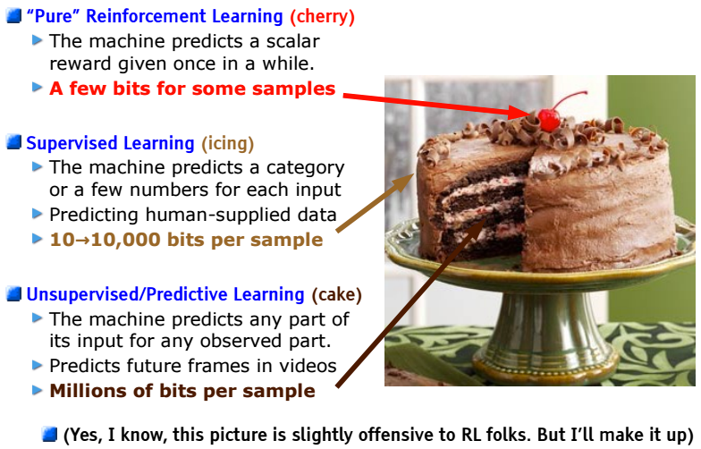
In the beginning of the conference, Yann LeCun gave a keynote, which may be considered a program speech for the whole conference. Besides starting the layered cake meme, he mentioned two ideas that he considers brightest in the last decade: adversarial training and external memory. My perception is that the most frequent buzzwords at the conference are:
  • generative adversarial networks (GAN),
  • recurrent neural networks (RNN),
  • reinforcement learning (RL),
  • robotics (done with or without RL).
Great engineers are good at defining useful abstractions. This LeCun’s layered cake metaphor was heavily re-used throughout the conference.
Andrew Ng gave a keynote on the workflow of applied DL research. Most ideas are trivial, although are often neglected. Here are a few of them. The most important metrics to track are: human error, training set error, and validation error. The gap between human and training set error is the bias. It can be solved by a bigger model or longer training. The validation/training gap is due to the variance. Once the bias problem is addressed, you can add more data or increase regularisation to reduce variance.

In practice, however, we have a different distribution of test data than of the training data. In that case, you might want to have two validation sets: one coming from training distribution, and another from test distribution. If you don’t have the latter, you will be solving a wrong problem. Domain adaptation methods may be also helpful, but are not quite practical at the moment.
He also heavily advocates for using the centralised data storage infrastructure that is easily available to all team members. It speeds up the progress a lot.
Currently, supervised learning dominates the landscape, while unsupervised and reinforcement learning are around for some time, but still cannot take off. Ng predicts that the second-biggest areas (after SL) will be not one of those, but transfer learning and multi-task learning. Those are important practical areas almost ignored by academic researchers.

There were seemingly few papers on architectural design (for supervised learning). Daniel Sedra gave a great talk on Neural networks of stochastic depth. The idea is to drop entire layers during training in ResNet-like architectures. That allows to grow them up to 1000+ layers, which gives significant improvement in accuracy on CIFAR (and not quite significant on ImageNet). Unfortunately, at test-time layers are there, so the inference time may be a problem. Another improvement is to add identity connection between each pair of layers, which also helps a bit.

Michael Figurnov, my academic sibling, presented a work on speeding up inference using so-called perforated convolutions. The idea is to skip some multiplications that do not impact the result of the operation a lot. In the follow-up work, he and co-authors suggest to skip the whole parts of the computation graph once they are estimated to be unimportant. This can potentially lead to significant speed-up, but for most practitioners it is the question of support in libraries such as CUDNN. Hopefully, we’ll be able to use it soon.
The method suggest not to waste computation time on background, but evaluate more ResNet layers where it can pay out more.
There was a demo I missed that demonstrated real-time object detection on a mobile device (if you have a link, please share with me!). It is based on YOLO, and the idea is to pre-compute and memoize some parts of the computational graph, then at inference time find the best approximation. There is some loss in accuracy, but real-time inference on the board looks impressive! 

The most interesting improvement for deep learning optimisation seems to be Weight normalisation. The paper builds on the idea of batch normalisation. It tries to explain the positive effect of it (i.e. staying on the unit sphere) and uses this intuition to propose an alternative way to stabilise the training process.

As I said above, GANs are a big (and controversial) topic here. It seems to be the most popular generative model for images, although variational autoencoders are still around. The training process is quite unstable, but the community is increasingly finding the ways to stabilise it. Most of them are hacks born in trial-and-error process. Soumith Chintala presented a list of 15 tricks in his talk How to train GAN? He promised to publish the slides later, but here is the writeup. If you will have to train GANs, make sure you read that first. There is no way you can guess this combination yourself (and papers typically do not mention all those hacks).
Poster by Soumith. TL;DR: use magic.
In the visual search field, there is a Universal correspondence network paper. Instead of matching features, it suggests to run one pass through the network to find dense correspondences. They claim that in comparison to extracting deep features for patches, the number of distance computations gets down from quadratic to linear (although, spatial index can also mitigate the issue). It appears to learn some notion of geometry/topology, i.e. one can train it to do rigid matching, as well as to look more at semantic similarity. The results they showed were on very similar images, so did not impress me much. Although it may had been done only to ease the visualisation.
Deep learning continues to disrupt traditional computer-vision pipelines.
For reinforcement learning, there is no single paper that I can pick as brightest, but the most impact seems to be done by publishing OpenAI Universe and DeepMind Lab, both are training environments for reinforcement learning algorithms stemming from computer-generated imagery (i.e. video games). It seems to be a valid step towards building intelligent agents operating in the real world, although there is a scepticism that it will be difficult to make the final step: the methods are data-hungry, and it is difficult to get a lot of data from anything rather than simulated environment, let alone having a frequent reward signal. This is one of the reasons researchers study the possibility of imitation learning, where a robot learns the cost function from demonstrations rather than taking it for granted. With this approach, we may be able to teach robots to perform tasks like pouring water into a glass by having a person or another robot showing it how to do it.
DeepMind collaborated with Blizzard to provide StarCraft API to facilitate training of RL agents. Now you have an excuse to play games at work.
Bayesian methods seem to be quite popular, and apparently can be successfully combined with neural networks (variational autoencoders and their variants are used a lot). Workshops on approximate variational inference and Bayesian deep learning have seen a large number of papers. Tutorial on variational inference (slides-pdf-1, slides-pds-2) reflected a significant progress in the recent years: things like reparametrisation trick and stochastic optimisation made possible to perform estimation of quite sophisticated posterior distributions. 
Slide by David Blei. Bayesian models have been long used successfully to estimate uncertainty, in particular to glue models to get complex pipelines while avoiding information loss. It is great we can use it with modern models as well.
Surely, an important part of the conference is socialisation. So thanks to everybody I had a chance to meet at the conference and had a productive (or just fun) conversation with. See you at the future conferences!

Read Users' Comments (9)

Launching Jupyter notebook server on startup

In this post, I show how to automatically run the Jupyter notebook server on an OSX machine on startup, without using extra terminal windows.

Background

Jupyter notebooks provide a useful interactive environment (think better alternative for console) for scripting languages like Python, Julia, Lua/torch, which has become a favourite tool of many data scientists for handling datasets that fit into the laptop’s memory. If you have not used it, try it next time you do data analysis or prototype an algorithm.

The Pain

There is a slight technical difficulty, though. The way Jupyter works is you run a server process on your machine (or somewhere in the network), and then access it through a web client. I have noticed a popular pattern of usage in the local-server case: a user runs the command to start the server process in the terminal then keeps the terminal window open while she is using the notebook. This method has several flaws:

  • you need to run the process manually each time you need a notebook (after reboot);
  • you have to remember the command line arguments;
  • the process takes up a terminal window/tab, or, if you run it in the background, you can accidentally close the tab and your RAM state will be lost.

The Solution

If your perfectionist’s feelings are hurt by those nuisances above, my setup may remedy it. It uses launchd framework that starts, stops, and manages background processes. 

First, create a property list file in your ~/Library/LaunchAgents directory: 

~/Library/LaunchAgents/com.blippar.jupyter-ipython.plist

and put the following text there. This is a custom format, which is not quite XML (e.g. order of children nodes apparently matters). I highlighted red the paths and other variables you will have to change:

<?xml version="1.0" encoding="UTF-8"?>
 <!DOCTYPE plist PUBLIC "-//Apple//DTD PLIST 1.0//EN"
  "http://www.apple.com/DTDs/PropertyList-1.0.dtd">
      <plist version="1.0">
      <dict>
          <key>KeepAlive</key>
          <true/>
          <key>Label</key>
          <string>com.blippar.jupyter-ipython</string>
          <key>ProgramArguments</key>
          <array>
              <string>zsh</string>
              <string>-c</string>
              <string>source ~/.zshrc;workon py3;jupyter notebook --notebook-dir /Users/roman/jupyter-nb --no-browser</string>
          </array>
          <key>RunAtLoad</key>
          <true/>
          <key>StandardErrorPath</key>
          <string>/Users/roman/Library/LaunchAgents/jupyter-notebook.stderr</string>
          <key>StandardOutPath</key>
          <string>/Users/roman/Library/LaunchAgents/jupyter-notebook.stdout</string>
      </dict>
      </plist>
     
The most interesting part is the ProgramArguments entry. As it is impossible to specify several commands as an argument, I had to run a separate shell instance and pass the commands separated by semicolons. If you do not need to set the virtual environment (workon py3), you might get away without calling the shell, although I recommend always using virtualenv for python on a local machine. Also, I use zsh; replace it with your shell of choice.

To check if everything works, run
launchctl load com.blippar.jupyter-ipython
launchctl start com.blippar.jupyter-ipython

and open http://localhost:8888/tree in your browser. Hopefully, you see the list of available notebooks.

Linux users, you should be able to replicate this with systemd (although, chances are you already know that =).

Read Users' Comments (6)

Asynchronous Fitter design pattern for training in IPython notebooks

[Cross-posted from CodeReview@SX]

The problem

When you work with Python interactively (e.g. in an IPython shell or notebook) and run a computationally intensive operation like fitting a machine-learning model that is implemented in a native code, you cannot interrupt the operation since the native code does not return execution control to the Python interpreter until the end of the operation. The problem is not specific to machine learning, although it is typical to run a training process for which you cannot predict the training time. In case it takes longer that you expected, to stop training you need to stop the kernel and thus lose the pre-processed features and other variables stored in the memory, i.e. you cannot interrupt only a particular operation to check a simpler model, which allegedly would be fit faster.

The solution

I propose an Asynchronous Fitter design pattern that runs fitting in a separate process and communicates the results back when they are available. It allows to stop training gracefully by killing the spawned process and then run training of a simpler model. It also allows to train several models simultaneously and work in the IPython notebook during model training. Note that multithreading is probably not an option, since we cannot stop a thread that runs an uncontrolled native code.

Here is a draft implementation:
from multiprocessing import Process, Queue
import time

class AsyncFitter(object):
    def __init__(self, model):
        self.queue = Queue()
        self.model = model
        self.proc = None
        self.start_time = None

    def fit(self, x_train, y_train):
        self.terminate()
        self.proc = Process(target=AsyncFitter.async_fit_, 
            args=(self.model, x_train, y_train, self.queue))
        self.start_time = time.time()
        self.proc.start()

    def try_get_result(self):
        if self.queue.empty():
            return None

        return self.queue.get()

    def is_alive(self):
        return self.proc is not None and self.proc.is_alive()

    def terminate(self):
        if self.proc is not None and self.proc.is_alive():
            self.proc.terminate()
        self.proc = None

    def time_elapsed(self):
        if not self.start_time:
            return 0

        return time.time() - self.start_time

    @staticmethod
    def async_fit_(model, x_train, y_train, queue):
        model.fit(x_train, y_train)
        queue.put(model)

Usage

It is easy to modify a code that uses scikit-learn to adopt the pattern. Here is an example:
import numpy as np
from sklearn.svm import SVC

model = SVC(C = 1e3, kernel='linear')
fitter = AsyncFitter(model)
x_train = np.random.rand(500, 30)
y_train = np.random.randint(0, 2, size=(500,))
fitter.fit(x_train, y_train)

You can check if training is still running by calling fitter.is_alive() and check the time currently elapsed by calling fitter.time_elapsed(). Whenever you want, you can terminate() the process or just train another model that will terminate the previous one. Finally, you can obtain the model by try_get_result(), which returns None when training is in progress.

The issues

As far as I understand, the training set is being pickled and copied, which may be a problem if it is large. Is there an easy way to avoid that? Note that training needs only read-only access to the training set.

What happens if someone loses a reference to an AsyncFitter instance that wraps a running process? Is there a way to implement an asynchronous delayed resource cleanup?

Read Users' Comments (3)

X Bridges of Königsberg

The recent Spiked Math comic strip proposes some cheats to build an Eulerian path over the famous bridges of Königsberg, which was originally impossible. Here is the strip:


It turns out that in practice another solution worked out (in fact, the mix of the engineer’s and mythbuster’s solutions). You can ruin the city during a world war and then transfer it to Russians, who will build the new bridges instead. I’ve been to Kaliningrad (the city has been renamed too) two years ago, but did not try to solve the Euler’s problem in field. Let’s find out if it is possible now. Look at the modern map:

View Königsberg bridges in a larger map

So, the modified Spiked Math’s scheme looks as follows (the new bridges are shown in light blue):

Is there an Eulerian path nowadays, i.e. can you walk through the city and cross each bridge once and only once? Recall the theorem:
A connected graph allows an Eulerian path if and only if it has no more than two vertices of an odd degree.
In the picture above, two pieces of land have even number of incident bridges, while the Kneiphof island in the center has degree 3, and the left bank (in the bottom) has degree 5. This means that now Eulerian paths exist. Any such path should begin in the left bank and end in the island, or vice-versa. It may be a good idea to finish your journey near the grave of Immanuel Kant. :) However, there is no Eulerian conduit, i.e. closed Eulerian path.

PS. 1. If you zoom out the above map, you’ll see one more piece of land and two more bridges on the East. However, it only adds a vertex of degree 2, and swaps parity of the banks, so the properties of the new graph are similar, you just need to start/finish your journey in the right bank, not the left one (and walk 10 km more).
2. When I was preparing this article, I found a similar analysis. It used an old map, so the Jubilee bridge and the 2nd Estacade bridges were not marked (they were built in 2005 and 2012, respectively), and also ignored the Reichsbahnbrüke (railroad bridge, but seems pedestrian-accessible).
3. It would be more interesting to analyze the bridge graphs of other cities with more islands like St. Petersburg (several hundred bridges) or Amsterdam (numerous bridges/canals, but have structure).
4. Here is Euler’s original paper (in Latin) with his drawings of the above schemes.

Read Users' Comments (34)

Machine learning in facebook

Last week Max Gubin gave a talk on how Facebook exploits machine learning. The talk was more technical then one might had expected, so I share some interesting facts in this posts. I hope it doesn’t disclose any secret information. :)

Max started with a screenshot of the Facebook interface, where each element was highlighted as beneficial of machine learning. Just to name some, they use learning to predict the order of stories in the newsfeed, groups/ads/chat contacts to show you, and even occasions when your account is supposedly hacked, so you need to verify your identity. For most of the tasks learning is probably trivial, but at least two of them involve complicated algorithms (see below).

Facebook engineers face number of difficulties. A user expects to load a page almost instantly, though network infrastructure already imposes some lag. To avoid further delaying, prediction should be done in tens of microseconds. Moreover, half a billion of daily-active users send a lot of queries, so massively-parallel implementations would be too expensive. They have no choice other than sticking to linear models. For example, they train a linear fitness function to rank the stories for the newsfeed (using e.g. hinge loss or logistic loss). It should be trained to satisfy multiple criteria, often contradicting. For example, maximizing personal user experience (showing most interesting stories) might hurt experience of other users (if one has few friends, they are the only users who can read his/her posts) or degrade the system as a whole (showing certain types of news might be not really interesting to anyone, while necessary to improve connectivity of the social network). Those criteria should be balanced in the learning objective, and the coefficients are changing over time. Even the personal user experience cannot be measured easily. The obvious thing to try is to ask users to label interesting stories (or use their Likes). However, such tests are always biased: Facebook tried to use this subjective labelling three times, and all of them were unsuccessful. Users just don’t tell what they really like.

Another challenge is the quickly-changing environment. For example, interest to specific ads may be seasoned. In advertising, one of the strategies is to maximize the click-through rate (CTR). The model for personalized ads should be able to learn online to adapt to changes efficiently. They use probit regression, where online updates can be written in a closed form, unlike to logistic regression (note the linear model again!). It is based on Microsoft’s TrueSkill™ method for learning ranks of players to find good matches and seems similar to what Bing uses for CTR maximization [Graepel et al., 2010].

Finally, Max mentioned the problem of estimating new features. The common practice in the industry is A/B testing, where a group of users is randomly selected to test some feature, and the rest of users are treated as the control group. Then they compare the indicators for those two groups (e.g. average time spent on the website, or clicks made on the newsfeed stories) and apply statistical tests. As usual, samples are typically small. For example, if they want to test a feature for search in Chinese, they take a small group of 10 million users, and hope that some of them will query in Chinese (recall that Facebook is unavailable in China). It is typically hard to prove a statistically significant improvement.

It was partially a hiring event. If you are looking for an internship or a full-time job, you may contact to their HR specialist in Eastern Europe Marina. Facebook also keeps in touch with universities, e.g. invites professors to give talks in their office or develop joint courses. Professors may apply, but I don’t know a contact for that.

Read Users' Comments (18)

PGM-class and MRF parameter learning

I’m taking Stanford CS 228 (a.k.a. pgm-class) on Coursera. The class is great, I guess it provides close to the maximum one can do under the constraints of remoteness and bulkness. The thing I miss is theoretical problems, which were taken aside from the on-line version because they could not be graded automatically.

There is an important thing about graphical models I fully realized only recently (partly due to the class). This thing should be articulated clearly in every introductory course, but is often just mentioned, probably because lecturers consider it obvious. The thing is there is no probabilistic meaning of MRF potentials whatsoever. The partition function is there not only for amenity: in contrast to Bayesian networks, there is no general way to assign potentials of an undirected graphical model to avoid normalization. The loops make it impossible. The implication is one should not assign potentials by estimating frequencies of assignments to factors (possibly conditioned on features) like I did earlier. This is quite a bad heuristic because it is susceptible to overcounting. Let me give an example.

For the third week programming assignment we needed to implement a Markov network for handwriting OCR. The unary and pairwise potentials are somewhat obvious, but there was also a task to add ternary factors. The accuracy of the pairwise model is 26%. Mihaly Barasz tried to add ternary factors with values proportional to trigram frequencies in English, which decreased performance to 21% (link for those who have access). After removing pairwise factors, the performance rose to 38%. Why has the joint model failed? The reason is overcounting evidence: different factor types enforce the same co-occurrences, thus creating bias towards more frequent assignments, and this shows it can be significant. Therefore, we should train models with cycles discriminatively. 

One more thought I’d like to share: graphical model design is similar to software engineering in the way that the crucial thing for the both is eliminating insignificant dependencies on the architecture design stage. 

Read Users' Comments (8)

When and why it is safe to cast floor/ceil result to integer

Happy new year, ladies and gents! I am back, and the following couple of posts are going to be programming-related.

The C/C++ standard library declares floor function such that it returns a floating-point number:
     double floor (      double x );
      float floor (       float x );  // C++ only
I used to be tortured by two questions:

  1. Why would the floor function return anything other than integer?
  2. What is the most correct way to cast the output to integer?

At last I figured out the answer to both questions. Note that the rest of the post applies to the ceil function as well.

For the second point, I knew the common idiom was just type-casting the output:

double a;
int intRes = int(floor(a));  // use static_cast if you don't like brevity
If you’ve heard anything about peculiarities of floating-point arithmetic, you might start worrying that floor might return not exact integer value but  $\lfloor a \rfloor - \epsilon$, so that type-casting is incorrect (assume $a$ is positive). However, this is not the case. Consider the following statement.

If $a$ is not integer and is representable as IEEE-754 floating-point number, than both $\lfloor a \rfloor$ and $\lceil a \rceil$ are representable within that domain. This means that for any float/double value floor can return a number that is integer and fits in float/double format.

The proof is easy but requires understanding of representation of floating-point numbers. Suppose $a = c \times b^q, c  \in [0.1, 1)$ has $k$ significant digits, i.e. $k$-th digit after the point in $c$ is not null, but all the further ones are. Since it is representable, $k$ is less then the maximum width of significand. Since $a$ is not integer, both $\lfloor a \rfloor$ and $\lceil a \rceil$ have significands with the number of significant digits less then $k$. Rounding however might increase the order of magnitude but only by one. So, the rounded number’s significand fits in $k$ digits, Q.E.D.

However, this does not mean one can always type-cast the output safely, since, for example, not every integer stored in double can be represented as 4-byte int (and this is the answer to the question #1). Double precision numbers have 52 digit significands, so any integer number up to $2^{52}$ can be stored exactly. For the int type, it is only $2^{31}$. So if there is possibility of overflow, check before the cast or use the int64 type.

On the other hand, a lot of int’s cannot be represented as floats (also true for int64 and double). Consider the following code:
std::cout << std::showbase << std::hex 
      << int(float(1 << 23)) << " " << int(float(1 << 24)) << std::endl
      << int(float(1 << 23) + 1) << " " << int(float(1 << 24) + 1) << std::endl;
The output is:

0x800000 0x1000000
0x800001 0x1000000

$2^{24}+1$ cannot be represented as float exactly (it is represented as $2^{24}$), so one should not use the float version of floor for numbers greater than few millions.

There are classes of numbers that are guaranteed to be represented exactly in floating point format. See also the comprehensive tutorial on floating-point arithmetic by David Goldberg.

Read Users' Comments (3)

Kinect Apps Challenge

Graphics & Media Lab and Microsoft Research Cambridge have announced a contest for applications that use Kinect sensor. The authors of the five brightest apps will be funded to attend the 2012 Microsoft Research PhD summer school. I blogged about the last year's event in my previous post. Details of the contest are here.

I guess there's no need to explain what Kinect is. It is extremely successful combined colour and depth sensor by Microsoft. It is being distributed for killer price (≈$150) as an add-on for Xbox, although it is hard to imagine the range of possible applications. Controlling a computer only by gestures is considered as a primer of natural user interface. To name some applications beyond gaming, this kind of NUI is useful to help surgeons to keep their hands clean:

Kinect helps blind people to navigate through buildings:

For more ideas look at the winners of OpenNI challenge.

OpenNI is an open-source alternative to Kinect SDK. Its strong point is it is integrated with PCL, but beware that you cannot use it for the contest. Only Kinect for Windows SDK is allowed.

Kinect is probably the most successful commercial outcome from the Microsoft Research lab. MSR is unique because they do a lot of theoretical research there, and it is unclear if it is profitable for Microsoft to fund it. But the projects like Kinect reveal the doubts. I will post about MSR organization in comparison to other industrial labs in one of the later posts.

Read Users' Comments (2)

All the summer schools

This summer I attended two conferences (3DIMPVT, EMMCVPR) and two summer schools. I know my latency is somewhat annoying, but it's better to review them now then never. :) This post is about the summer schools, and the following is going to be about the conferences.


PhD Summer School in Cambridge

Both schools were organized by Microsoft Research. The first one, PhD Summer School was in Cambridge, UK. The lectures covered some general issues for computer science PhD students (like using cloud computing for research and career perspectives) as well as some recent technical results by Microsoft Research. From the computer vision side, there were several talks:
  • Antonio Criminisi described their InnerEye system for retrieval of similar body part scans, which is useful for diagnosis based on similar cases' medical history. He also featured the basics of Random Forests as an advertisement to his ICCV 2011 tutorial. The new thing was using peculiar weak classifiers (like 2nd order separation surfaces). Antonio argued they perform much better then trees in some cases.
  • Andrew Fitzgibbon gave a brilliant lecture about pose estimation for Kinect (MSR Cambridge is really proud of that algorithm [Shotton, 2011], this is the topic for another post).
  • Olga Barinova talked about the modern methods of image analysis and her work for the past 2 years (graphical models for non-maxima suppression for object detection and urban scene parsing).
The other great talks were about .NET Gadgeteer, the system for modelling and even deployment of electronic gadgets (yes, hardware!), and F#, Microsoft's alternative to Scala, the language that combines object-oriented paradigm with functional. Sir Tony Hoare also gave a lecture, so I had a chance to ask him how he ended up in Moscow State University in the 60s. It turns out he studied statistics, and Andrey Kolmogorov was one of the leaders of the field that time, so that internship was a great opportunity for him. He said he had liked the time in Moscow. :) There were also magnificent lectures by Simon Peyton-Jones about giving talks and writing papers. Those advices are the must for everyone who does research, you can find the slides here. Slides for some of the lectures are available from the school page.

The school talks did not take all the time. Every night was occupied by some social event (go-karting, punting etc.) as well as unofficial after-parties in Cambridge pubs. Definitely it is the most fun school/conference I've attended so far. Karting was especially great, with the quality track, pit-stops, stats and prizes, so special thanks to Microsoft for including it to the program!


Microsoft Computer Vision School in Moscow

This year, Microsoft Research summer school in Russia was devoted to computer vision and organized in cooperation with our lab. The school started before its official opening with a homework assignment we authored (I was one of four student volunteers). The task was to develop an image classification method capable to distinguish two indoor and two outdoor classes. The results were rated according to the performance on the hidden test set. Artem Konev won the challenge with 95.5% accuracy and was awarded a prize consisted of an xBox and Kinect. Two years ago we used those data for the projects on Introduction to Computer Vision course, where nobody reached even 90%. It reflects not just the lore of participants, but also the progress of computer vision: all the top methods used PHOW descriptors and linear SVM with approximate decomposed χ2 kernel [Vedaldi and Zisserman, 2010], which were unavailable that time!

In fact, Andrew Zisserman was one of the speakers. Andrew is the most cited computer vision researcher and the only person whose Zisserman number is zero. :) His course was on Visual Search and Recognition, including instance-level and category-level recognition. The ideas that were relatively new:
  • when computing visual words, sometimes it is fruitful to use soft assignments to clusters, or more advanced methods like Locality-constrained linear coding [Wang et al., 2010];
  • for instance-level recognition it is possible to use query expansion to overcome occlusions [Chum et al., 2007]: the idea is to use the best matched images from the base as new queries;
  • object detection is traditionally done with sliding window, the problems here are: various aspect ratio, partial occlusions, multiple responses and background clutter for substantially non-convex objects;
  • for object detection use bootstrapped sequential classification: on the next stage take the false negative detections from the previous stage as negative examples and retrain the classifier;
  • multiple kernel learning [Gehler and Nowozin, 2009] is a hot tool that is used to find the ideal linear combination of SVM kernels: combining different features is fruitful, but learning the combination is not much better than just averaging (Lampert: “Never use MKL without comparison to simple baselines!”);
  • movies are common datasets, since there are a lot of repeated objects/people/environments, and the privacy issues are easy to overcome. The movies like Groundhog Day and Run Lola Run are especially good since they contain repeated episodes. You can try to find the clocks on Video Google Demo.
Zisserman talked about PASCAL challenge a lot. During a break he mentioned that he annotated some images himself since “it is fun”. One problem with the challenge is we don't know if the progress over years really reflects the increased quality of methods, or is just because of growth of the training set (though, it is easy to check).

Andrew Fitzgibbon gave two more great lectures, one about Kinect (with slightly different motivation than in Cambridge) and another about continuous optimization. He talked a lot about reconciling theory and practice:
  • the life-cycle of a research project is: 1) chase the high-hanging fruit (theoretically-sound model), 2) try to make stuff really work, 3) look for the things that confuse/annoy you and fix them;
  • for Kinect pose estimation, the good top-down method based on tracking did not work, so they ended up classifying body parts discriminatively, temporal smoothing is used on the late stage;
  • “don't be obsessed with theoretical guarantees: they are either weak or trivial”;
  • on the simplest optimization method: “How many people have invented [coordinate] alternation at some point of their life?”. Indeed, the method is guaranteed to converge, but the problems arise when the valleys are not axis-aligned;
  • gradient descent is not a panacea: in some cases it does small steps too, conjugate gradient method is better (it uses 1st order derivatives only);
  • when possible, use second derivatives to determine step size, but estimating them is hard in general;
  • one almost never needs to take the matrix inverse; in MATLAB, to solve the system Hd = −g, use backslash: d = −H\g;
  • the Friday evening method is to try MATLAB fminsearch (implementing the derivative-free Nelder-Mead method).
Dr. Fitzgibbon asked the audience what the first rule of machine learning is. I hardly helped over replying “Never talk about machine learning”, but he expected the different answer: “Always try the nearest neighbour first!”

Christoph Lampert gave lectures on kernel methods, and structured learning, and kernel methods for structured learning. Some notes on the kernel methods talk:
  • (obvious) don't rely on the error on a train set, and (less obvious) don't even report about it in your papers;
  • for SVM kernels, in order to be legitimate, a kernel should be an inner product; it is often hard to prove it directly, but there are workarounds: a kernel can be drawn from a conditionally positive-definite matrix; sum, product and exponent of a kernel(s) is a kernel too etc. (thus, important for multiple-kernel learning, linear combination of kernels is a kernel);
  • since training (and running) non-linear SVMs is computationally hard, explicit feature maps are popular now: try to decompose the kernel back to conventional dot product of modified features; typically the features should be transformed to infinite sums, so take first few terms [Vedaldi and Zisserman, 2010];
  • if the kernel can be expressed as a sum over vector components (e.g. χ2 kernel $\sum_d x_d x'_d / (x_d + x'_d)$), it is easy to decompose; radial basis function (RBF) kernel ($\exp (\|x-x'\|^2 / 2\sigma^2)$) is the exponent of a sum, so it is hardly decomposable (more strict conditions are in the paper);
  • when using RBF kernel, you have another parameter σ to tune; the rule of thumb is to take σ² equal to the median distance between training vectors (thus, cross-validation becomes one-dimensional).
Christoph also told a motivating story why one should always use cross-validation (so just forget the previous point :). Sebastian Nowozin was working on his [ICCV 2007] paper on action classification. He used the method by Dollár et al. [2005] as a baseline. The paper reported 80.6% accuracy on the KTH dataset. He outperformed the method by a couple of per cents and then decided to reproduce Dollár's results. Imagine his wonder when simple cross-validation (with same features and kernels) yielded 85.2%! So, Sebastian had to improve his method to beat the baseline.

I feel I should stop writing about the talks now since the post grows enormously long. Another Lampert's lecture and Carsten Rother's course on CRFs were close to my topic, so they deserve separate posts (I already reviewed basics of structured learning and max-product optimization in this blog). Andreas Müller blogged about the recent Ivan Laptev's action recognition talk on CVML, which was pretty similar to ours. The slides are available for all MSCVS talks, and videos will be shared in September.

There were also several practical sessions, but I personally consider them not that useful, because one hardly ever can feel the essence of a method in 1.5 hours changing the code according to some verbose instruction. It is more of an art to design such tutorials, and no one can really master it. :) Even if the task is well-designed, one may not succeed performing it due to technical reasons: during Carsten Rother's tutorial, Tanya and me spent half an hour to spot the bug caused by confusing input and index variable names (MATLAB is still dynamically typed). Ondrej Chum once mentioned how his tutorial was doomed since half of the students did not know how to work with sparse matrices. So, practical sessions are hard.

There was also a poster session, but I cannot remember a lot of bright works, unfortunately. Nataliya Shapovalova who won the best poster award, presented quite interesting work on action recognition, which I liked as well (and it is not the last name bias! :) My congratulations to Natasha!

The planned social events were not so exhaustive as in Cambridge, but self-organization worked out. The most prominent example was our overnight walk around Moscow, in which a substantial part of school participants took part. It included catching last subway train, drinking whiskey and gin, a game of guessing hallucinating names of each other, and moving a car from the tram rail to let the tram go in the morning. :) I also met some of OpenCV developers from Nizhny Novgorod there.


MSCVS is a one-time event, unfortunately. There are at least three annual computer vision summer schools in Europe: ICVSS (the most mature one, I attended it last year), CVML (held in France by INRIA) and VSSS (includes sport sessions besides the lectures, held in Zürich). If you are a PhD student in vision (especially in the beginning of your program), it is worth attending one of them each year to keep up with current trends in the vision community, especially if you don't go to the major conferences. The sets of topics (and even speakers!) have usually large intersection, so pick one of them. ICVSS has arguably the most competitive participant selection, but the application deadline and acceptance notification are in March, so one can apply to the other schools if rejected.
Read Users' Comments (7)